/ Interface / Graphical Plots

Fiddle allows you to visualize intricacies of your ChucK compositions by scanning for special OSC messages produced as your compositions run. The Plot Panel supports multiple plotting surfaces and the Fiddle Runtime includes a number of nodes that route signals and events to the Plot Panel for your inspection.

Signal Plot

A signal plot depicts time-dependent values associated with an audio or control signal.

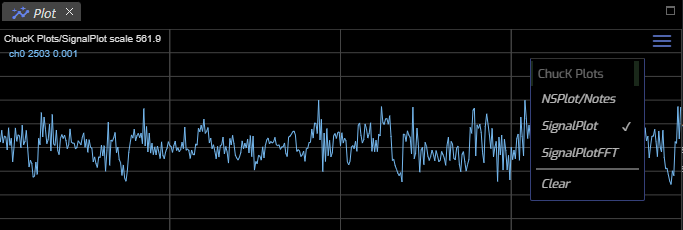
Note that a Plot Surfaces Menu is available by clicking on the menu in the upper right corner of the panel. In this case there are three plots, NSPlot/Notes and SignalPlot and SignalPlotFFT available in this panel.

Your ChucK compositions can trigger delivery of multiple plotting surfaces and this menu allows you to switch between them. In addition, a single plot can present multiple signals. In this example, we have a single signal, ch0 on the plot surface, SignalPlot. Since audio signals have a lot of dynamic range, it's common to need to scale the plot according to your signal strength. Here we've scaled the signal plot by 581, since the RMS is quite small in this example.

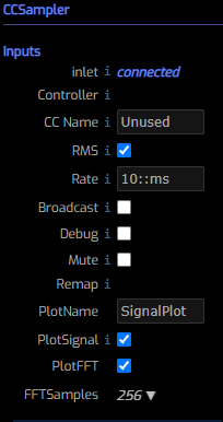
At right are the key parameters of the CCSampler Node that are found in this simple example. Other plotting nodes include CCPlot and NSPlot and are covered below.

As described elsewhere, CCSampler samples an incoming signal at a requested sampling rate. The result can be routed to a consumer of control signals and can also be plotted as a signal and/or as an FFT. If you select both, you'll get two distinct plotting surfaces due to the fact that the units of an FFT and a Signal plot aren't compatible.

Sometimes your incoming signal doesn't fit well within the default bounds of the plot. You can use your Mouse Wheel to modify the vertical axis scale. Typically values need to be greater than 1 to perceive the signal detail. When you have both PlotSignal and PlotFFT we generate an always positive RMS signal which is more accurate than the positive and negative signal-sample obtained when not computing the FFT. When viewing RMS signal values the scale factor must typically be larger still.

Spectrum

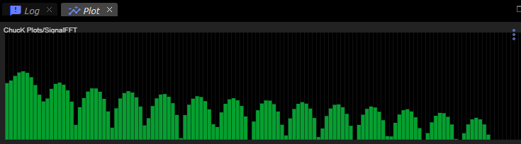
If you select PlotFFT and 1024 FFT samples you'll get something like this. The axes for a Spectrum plot are decibels on the y axis (ie: it's logarithmic) and linear frequency on the X axis.

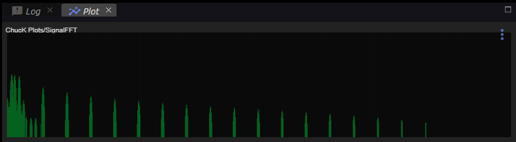
And here's one with 256 FFT samples (NB:this parameter can't be set "live"). You can choose an update rate with the CCSampler's Rate parameter. Try Rate values between 1::ms and 1::second to get a feel for its affect.

Note Plot (Piano Roll)

Note-plots like the following can be generated via the NSPlot node.

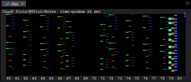
In this example, we see a range of MIDI notes from note 60 to note 80. Within each note-column are three channel-columns. This is the case because this example has three "pianos" all contributing to the same "roll".

Here, channel 0 produces green notes and these appear on the left-most side in each note-column that was touched by this channel. In this display older notes are at the top of the display and the newest notes are below older notes. So this piano roll scrolls from bottom to top.

Each colored rectangle represents a note. Taller notes were held for a longer time period. As with signal plots you can use the Mouse Wheel to control the scaling of the vertical axis. This is reflected in the value for time-window as shown at the top of the graph.

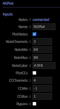
At right we see the parameters for a single NSPlot node. The Name field represents the plot surface that we'd like our notes to be associated with. Each of the three NSPlot nodes in this example have the same value for this parameter. The NoteChannels, NoteMin and NoteMax parameters configure the note plot and the values from the first channel requesting the plot surface are the values that are respected. Generally this values should be the same for all nodes targeting a shared plot surface if only to prevent confusion.

The NoteColor parameter can select the color of the notes that derive from this channel. You can use standard css color notation. Leaving the value empty will cause Fiddle to select a color randomly.

In addition to generating notestream plots, NSPlot offers the convenience of also generating CC signal plots. The key difference between signal plots that arise from NSPlot and CCPlot nodes from those produced by CCSampler is that the CC sampling rate is controlled elsewhere. And, while audio signals reside within the [-1, 1] value range CC values can take any values. The CCMin and CCMax values provide the default plotting range for the connected CC generator. The CCChannels is required to initialize a plot surface and represents the number of CCs that are expected for plotting. Since a single NoteStream connection can produce arbitrary CCs you may need to increase this value to visualize the CCs you want.

Box2D

The Box2D plotting surface presents a rendering of a Box2D world and is updated as the Box2D physics simulation proceeds within a running ChucK session. Here's an example of Box2D plot in action.

Controls

• Mouse-click/drag to pan
• Mouse-wheel to zoom
• Enable/Disable Ghosting via the menu icon at top-right.

Ghosting

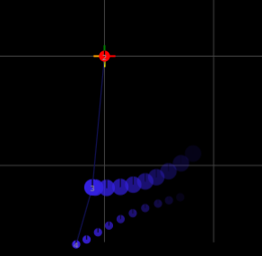
When enabled, ghosting draws a recent history of body locations in your scene. For complex scenes, this can result in drawing slowdowns or just too much slop. For simple pendula setups, there's no denying it, ghosting looks cool. For additional insight into your Box2D data, keep in mind that signal plots are a great way to focus on your control signals (eg the X channel of position or the velocity magnitude, etc).